A musical piece is usually represented by various musical elements drawn on the musical staff. ♫
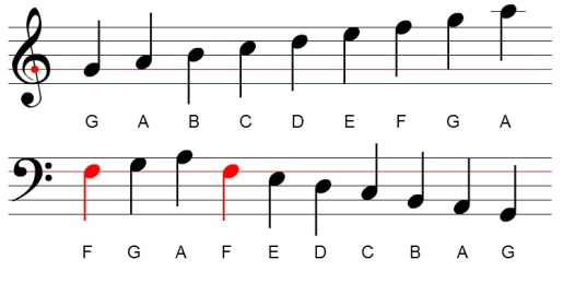
The staff is composed of five lines and four spaces. Each of these components represents a key or note. A clef is the first element seen from the left of a staff and it assigns the specific note to the lines or spaces. The most common clefs are the Treble or G clef and the Bass or F clef. The staff line for which a G clef encloses is named as G (Sol) whereas the staff line between the two dots of an F clef is F (Fa). The rest of the letter names follow. A ledger line is a little line that extends the staff when there is no more available line. The figure below shows the letter names of lines and spaces for a Treble and a Bass staff [1].
Figure 1. The Treble staff (top) and Bass staff (bottom) notations [1].
Combining the two staffs above, a Grand staff is formed. This extended staff is formed to avoid preposterous number of ledger lines. The letter between the two staffs is known as the Middle C. The Grand staff and its notation are shown below [2].
Figure 2. The Grand staff notation [2]
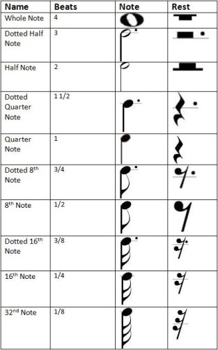
Having known the positions of the letter names, the notes and rests should be determined afterwards. These symbols suggest the corresponding number of beats. Figure 3 illustrates the different types of notes and rests.
Figure 3. Various types of notes and rests [3].
In this activity, we were tasked to play the notes in a digital image of a musical score sheet using Scilab (AMAZING, ISN’T IT?). This is done by extracting the notes and playing them with the corresponding frequency and duration [4]. I was greatly surprised that we can actually make Scilab “sing”!!!
The snippet shown below is an example of a code that can make Scilab “sing” the first line of the nursery rhyme “Mary had a little lamb”. It was given in the manual.
Figure 4. Mary had a little lamb Scilab code [4].
The lines and spaces on the staff which were discussed earlier correspond to specific notes in a heptatonic (7-note scale): do-re-mi-fa-sol-la-ti or C-D-E-F-G-A-B. These notes have their unique frequencies. Various musical elements also have unique durations. In this activity, Scilab will be used to produce the sinusoidal waves representing the series of notes in a musical piece. These waves will then be converted to sound by the speaker of the computer installed with this program [4].
It was written in the manual that any air vibration greater than 20 Hz and less than 22 kHz can be sensed by the human ear. Therefore, the rests can be represented by a frequency not equal to any value in the said range.
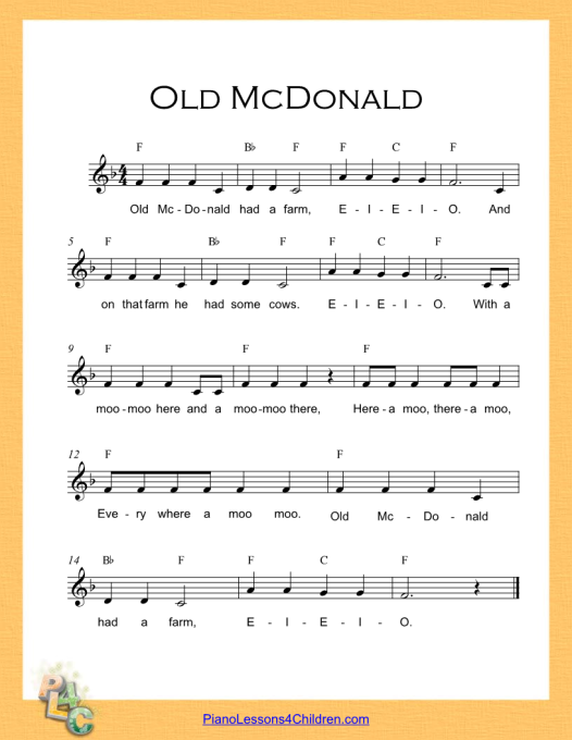
The first step of the activity is to find a simple musical score sheet image on the web. A simple score has only one note per column in the staff. I chose the nursery rhyme entitled “Old McDonald” and downloaded the musical score from reference [5]. The image of the musical score sheet is shown below.
Figure 5. Old McDonald F Major Musical sheet for Piano [5]
We can see from Figure 5 that Old McDonald in F Major sheet contains 56 notes, 2 rests and 3 dotted notes.
The second step is to make use of all the image processing techniques that I have learned from this course to determine the notes and the duration in the musical score. In this case, I have to determine the notes and the durations in the musical score from Figure 5.
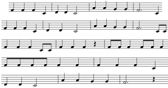
In order to optimize the image processing, I decided to crop the staff and remove the unnecessary information. I only need the notes and rests. The cropped image is shown below.
Figure 6. Cropped image of Figure 5.
After that, I thought of the steps and specific image processing techniques I need for the determination of the letter names and duration. The first thing that came to my mind is correlation (followed by digital scanning hehe) because these directly focused on the positions of pixels. I tried to avoid the use of mask/filter in this case because some pixels were removed. This happened in the previous activity. I do not want to lose any information and suppress the quality of the image as much as possible. Hence, I made the following steps as I organized my thoughts:
Convert image to binary using threshold values. This is done to make the image sharp and correlation will be more accurate.
Invert the image. It is because I’m thinking of using correlation to determine the position of notes/rest.
Apply morphological operations. I chose this to avoid similar shapes of notes and make distinct shapes.
Make templates of the existing notes/rest in the music sheet. The elements involve quarter note, half note, dotted half note, eighth note, quarter rest.
Execute correlation as the image processing technique. This is the method I think I can use to get the position of the templates (concept of FFT).
Store important values. Such values are note, x-position and y-position. Knowing the note means knowing the duration, y-position (which is a range) indicates the letter name (CDEFGAB) on the staff and x-position (which is a range also) suggests the sequence of the notes on the staff. The values are in ranges to compensate for the position and littleness of the pixels.
Enter the values to a time series. It will make the extraction of data easier. Sorting the values according to the values of x-position will make a time series of the notes.
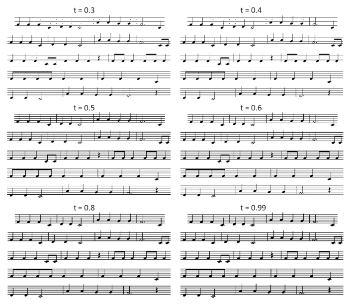
Figure 7 shows the binarized images of the cropped music score from Figure 6. First, I chose the enhanced image with 0.99 threshold value since the width of stems of the notes there were pretty much consistent with each other. But the correlation did not give a good results. I found out that the binary image with t = 0.5 is the preferable image.
Figure 7. Binarized image of Figure 5 for various threshold value (t= 0.3, 0.4,0.5, 0.6, 0.8, 0.99)
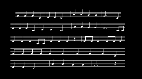
Figure 8 shows the inverted image of binarized image with t = 0.5 from Figure 7.
Figure 8. Inverted image from Figure 7 with t = 0.5.
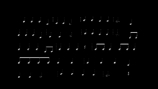
I applied the skel() function of Scilab as the morphological operation hoping that each type of the elements will be distinct from each other. In line with this, I can have an accurate result for correlation. The resulting morph-ed image is shown in Figure 9.
Figure 9. Skeletonized version of the image from Figure 8.
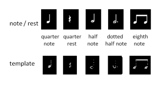
It can be observed from Figure 9 that the notes and the rest are distinct from each other. The next figure shows the various templates and the corresponding note/rest which they symbolize. These templates will later be used for correlation.
Figure 10. Templates and the musical elements they represent for correlation.
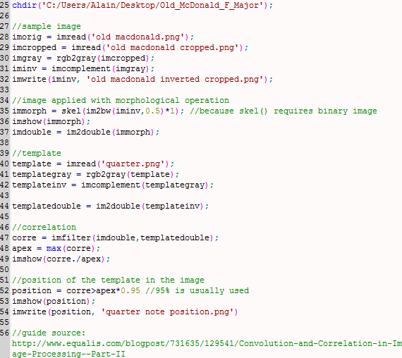
Now is the time to do the correlation. I believe we have completed an activity concerning correlation and convolution in image processing in AP 185 last semester. It is essentially a method of finding the positions in an image that matches the configuration of pixels of the template. By good fortune, I found a set of Scilab functions from reference [6] which performs the same process. Below is the Correlation code for finding the quarter note template in the cropped, binarized and skeletonized image of the sample music score shown in Figure 9. The same process works for other templates from Figure 10.
Figure 11. Scilab code for the Correlation technique
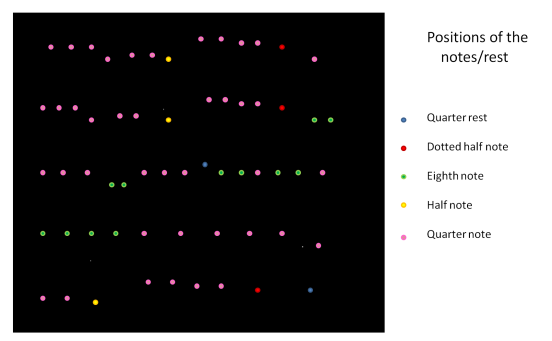
Upon performing such method, I got the following results. Note that I made separations between the staffs because it looked overfilled when presented in the original positions.
Figure 12. Positions of notes/rest acquired using Correlation
Once I got the position of a certain note/rest, I planned to use imconv() function (2D convolution) to change the white pixel indicating the position to another configuration. However, it is not working in my Scilab this time though my SIP toolbox and SIVP are working 😦 I wonder why. Hence, I just varied the pixel color for different notes/rest and represented them with circles.
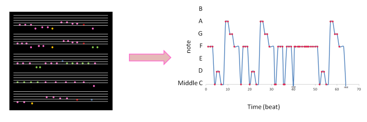
Each of the circles in Figure 12 has three important values: note (duration), x-position (beat) and y-position (letter name). For an orderly solution, these values are expressed in a time series shown below.
Figure 13. Time series of the note “values” (CDEFGAB).
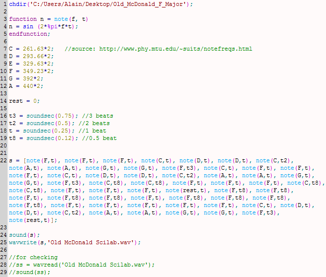
It will be easier to implement the data to a Scilab by consulting the time series above. The pink circular markers in the time series are the keys and the blue lines indicate the behavior of the keys. My Scilab code is shown below. The framework of this code was taken from Figure 4.
Figure 14. Old McDonald Scilab code
The third and last procedure is to check whether I got the notes and duration correctly. I have executed it by saving the tunes using wavwrite() function, checking it using wavread() function and then playing the tunes. Click the link to access the audio clip (Old McDonald Scilab.wav):
http://www.mediafire.com/?y42tdq85laxmv6d
I also made use of rests in the series of notes in the second procedure for the bonus part to faithfully follow the musical score. See Figure 14 for the code.
For me, this is the most interesting activity for this course this time! It exercised our knowledge from the past activities for it to be accomplished. I can tell that learning is really fun in this course!
In this case, I give myself a grade of 12/10 for doing every steps and for doing the bonus part.
References:
1. “The Staff, Clefs, and Ledger Lines”, retrieved from http://www.musictheory.net/lessons/10.
2. “Simplifying the Grand Staff”, retrieved from http://www.theoreticallycorrect.com/MusicFiction/new-grand-staff/index.html.
3. “Note/Rest Durations and Relationships”, retrieved http://4evatalent.wordpress.com/4evamusical/music-theory/noterest-durations-and-relationships/.
4. Maricor Soriano, “A9 – Applications of Morphological Operations 2 of 3: Playing notes by Image Processing”, 2012.
5. “Old McDonald”, retrieved from http://www.pianolessons4children.com/sheetmusic/Old_McDonald_F_Major.pdf.
6. “Convolution and Correlation in Image Processing – Part II”, retrieved from http://www.equalis.com/blogpost/731635/Scilab-Tips?tag=January.
7. “Frequencies for Equal-Tempered Scale”, retrieved from http://www.phy.mtu.edu/~suits/notefreqs.html.
