AP 186 Activity 12: Basic Video Processing

Video and Audio

Video and audio refer to storage formats for moving pictures and sound, respectively, which changes through time. Recording a video or audio is also known as video or audio codecs. Video codecs comprises of a series of images, or frames while audio codecs commonly comprises of a single channel or mono, two channels or stereo or more. The quality of videos depends upon the number of frames per second, the resolution of the images and the color space used. On the other hand, the number of bits per playback time, or bitrate, determines the quality of audio [1].

Video and audio are used to develop family videos, presentations, web pages and others. It is recommended by the Web content accessibility guidelines to provide alternatives for this kind of media like captions, descriptions or sign language when producing videos all the time [1].

Video and audio are formulated to improve experiential learning or entertainment.

Video is a series of still images presented in a fast succession so that there will be a perception of motion by the audience [2]. Observe the image below.

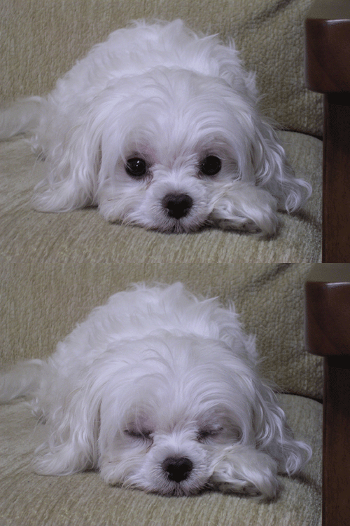
Figure 1. A GIF image of a dog [3].

A video can either be analog or digital. In this regard, the image processing techniques we have learned can be applied to the ‘still’ images. The frame rate for a digital is known as fps or frames per second. By taking the inverse of fps, we get the time interval between frames or the Δt [2].

This activity revolves around basic processing of a video. The audio here is omitted.

In particular, dynamics and kinematics of a specific system will be extracted from a video [2].

Important note: If an image seems to be indistinct, simply click that image for larger view. 😀

Kinematic Experiment

A video of a kinematic experiment, specifically 3D Spring Pendulum, is the subject for this activity.

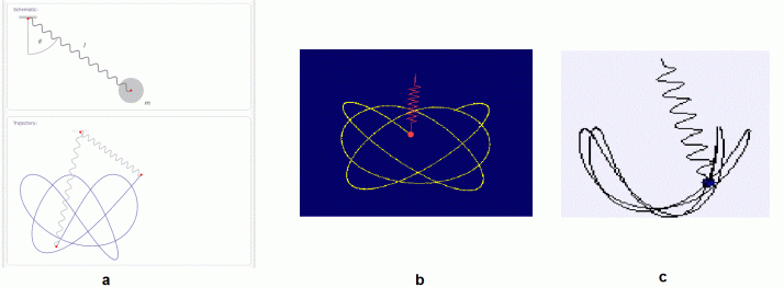
A 3D spring pendulum consists of a spring-mass system with three degrees of freedom. Having such, its behavior becomes chaotic. For a simple pendulum, the string length is constant giving rise to a constant period. However, the length of spring in a spring pendulum changes every time [4].  Below are some examples of chaotic behavior.

Figure 2. Chaotic behavior of two 3D spring pendulum systems. a from [4], b from [5] and c from [6].

Materials and Setup

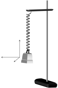
The materials used are iron rod, clamp, spring, 20 g mass (actually 19.1g), Canon D10 camera, tripod, FFmpeg software, laptop, red pentel pen and masking tape. The assemblage of the first four materials is  shown below.

Figure 3. 3D spring pendulum (drawn using MS Powerpoint).

The digital camera was used to take the video of the kinematics and the software for video processing. The red pentel pen and masking tape were used to ensure that the color of the mass is unmistakably different from the background.

Procedure

The first step is to take a video of the actual 3D spring pendulum system in motion. The video showing the system along the side of the setup can be found here:

http://www.mediafire.com/download.php?6xfzap395c99w6z

The frame rate of the video is actually 30 fps. FFmpeg was used to extract images from the video above. This program was ran using command prompt and following the format:

ffmpeg -i <filenameofimage> <filenameofsavedimage>

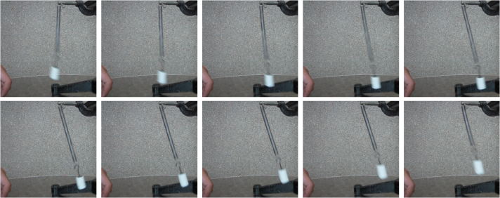
The 141st to 150th frames/images from the video are shown below.

Figure 4. Sample images extracted from the video above (141st to 150th frames).

Since the images were now extracted, image processing techniques can be executed. Here is my plan to get the position of the mass:

• loop through images
• image segmentation (parametric and non-parametric then choose the better one)
• get the pixel position of the centroid of the blob
• append the pixel positions to an array and plot the track of the mass in 2 dimensions

So the next thing I did was to do Image Segmentation. But here’s the problem: I found out that the iron rod was also included in the segmentation! 😦 Since the mass was white and specular reflection occurred in the iron rod, the segmented images contain the iron rod as well. I cropped out the image so that there will be no more problems. However, some of the pebbles were also included! 😦 I used FastStone Photo Resizer 3.1 to crop and edit the images by batch. We were not careful about the color of our subject that is why we have to deal with this problem.

Figure 5. Cropped version of the image from Figure 4.

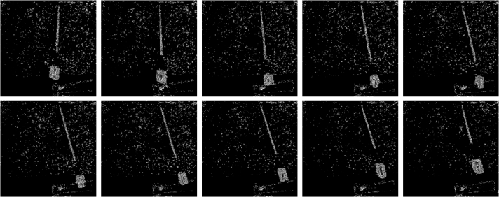
What I did was to segment the images first. The segmented version of the images from Figure 3 using parametric segmentation are shown below.

Figure 6. Parametrically segmented images corresponding to the images in Figure 5.

I thought of using morphological operations for the images above so that I can isolate the biggest blob. However, I still have another choice. That is, non-parametric segmentation. Figure 7 shows the corresponding segmented images using non-parametric segmentation.

Figure 7. Non-parametrically segmented images corresponding to the images in Figure 5.

By inspecting Figures 6 and 7, we can see that non-parametric segmentation produced better results so I used it for the next step. The next thing we need to do is to get the centroid of the ROI (region of interest) which is the mass so that we can know its pixel position in the image.

By the way, segmentation was done with ease because I looped through the images. 😀 The processing is simple but running the code took a very looooong time. The video’s length is 3 minutes 11 seconds but I only processed the first minute. That means I looped through 1800 images in order to produce both the parametrically and non-parameterically segmented images. 🙂

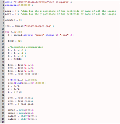
[Going back to the discussion] I made two empty arrays from the beginning of my code: posx and posy. See the last figure for my Scilab code. When the centroids of all the images were taken, the x and y positions are binned in posx and posy, respectively. In the end, posx and posy are plotted against each other. The result is actually the track plot and it is shown below.

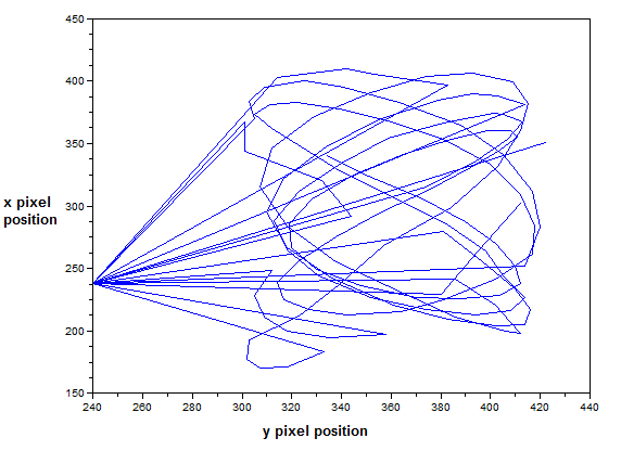
Figure 8. Track plot of the mass in the pendulum from the video above (170 frames).

The plot from Figure 8 shows the track of the mass using 170 frames only so that it will be presentable. Too much frames will show more lines that might conceal the directions. We can see from Figure 8 that the path of the mass is chaotic and similar to Figures 2a and 2b.

We took another video of the 3D spring pendulum but this time, its motion is viewed from the bottom of the setup. It can be found by clicking the following link:

http://www.mediafire.com/download.php?p86nd84r95zcjyh

The 141st to 150th frames are shown below.

Figure 9. Sample images from the second video (141st-150th frames).

I did not have a problem segmenting the images from this scene since the mass here is covered with masking tape applied with red pentel pen ink. (Thank God.) The parametrically segmented images corresponding to the 141st to 150th frames are shown below for sample images.

Figure 10. Parametrically segmentated images corresponding to the images from Figure 9.

and the non-parametrically segmented images are shown in the next figure.

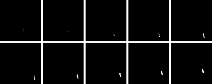
Figure 11. Non-parametrically segmented images corresponding to Figure 9.

Again, the non-parametrically segmented images were better than the parametrically segmented ones just like in the case of the first video. I then looped through the images and took their centroids to determine their positions per image. The plot of the positions are shown below.

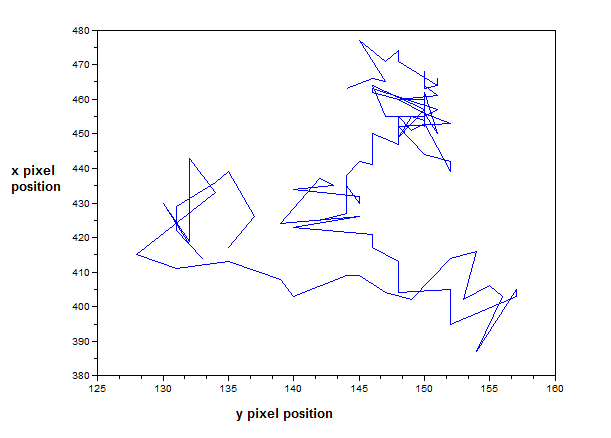
Figure 12. Track plot of the mass in the pendulum from the second video (100 frames).

The plot from Figure 12 shows the track using 100 frames only. Adding more frames will show more chaotic plot. Once again, the track of the mass is similar to the track illustrated in Figure 2. We can account the difference from the fact that it is not ideal and by presence of air drag, spring constant, initial force and other external forces.

On a side note, I thought of using correlation from the beginning instead of taking the centroid. This method, however, consumes too much memory and running time so I chose the determination of centroid in the end.

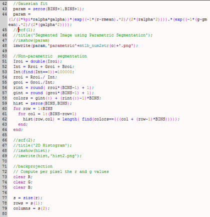
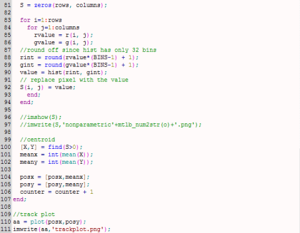
My whole code is shown below.

Thanks to my cooperative groupmates, Gino Borja and Tin Roque. We prepared the kinematics experiment and took the video together. Gino has introduced FFmpeg. We have thought of looking for the path/track of the mass together but we decided to choose our own way to attack the problem and create the programming codes on our own. We would like to thank the VIP group of IPL for lending their Canon D10 camera and a tripod. I would like to give myself a grade of 10 for doing all the steps.

This is the last activity for this course! Yey!! 😀 I can say that I really enjoyed this subject and I’ve learned a LOT about image processing and Scilab. This course also extended my imagination! 😀 Thank you!

References:

1. “Audio and Video”, retrieved from http://www.w3.org/standards/webdesign/audiovideo.html.

2. Maricor Soriano, “AP 186 Activity 12 Basic Video Processing”, 2012.

3. “Puppy/Dog Animations”, retrieved from http://longlivepuppies.com/PuppyDogPicture.a5w?vCategory=Gifs&bPostnum=00000000222.

4. “From Simple to Chaotic Pendulum Systems in Wolfram|Alpha”, retrieved from http://blog.wolframalpha.com/2011/03/03/from-simple-to-chaotic-pendulum-systems-in-wolframalpha/.

5. “Spring Pendulum”, retrieved from http://www.maths.tcd.ie/~plynch/SwingingSpring/springpendulum.html.

6. “EJs CM Lagrangian Pendulum Spring Model”, retrieved from http://www.compadre.org/osp/items/detail.cfm?ID=7357.

AP 186 Activity 11: Color Image Segmentation

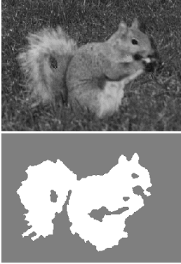
Image segmentation is an image processing technique where a region of interest (ROI) of an image is selected for further processing. It can be applied in grayscale images by means of getting the thresholding value [1] .The next figure shows an example

Figure 1. Grayscale image segmentation [2]

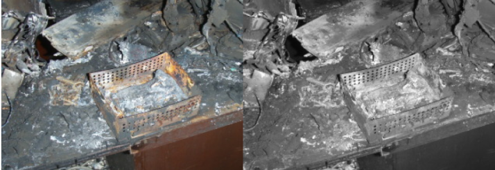
However, the desirable image sometimes cannot be obtained by thresholding. Say for example the ROI of an image has the same grayscale pixel value with the surrounding area. One cannot simply use thresholding for segmentation in this case. See the next figure for an example.

Figure 2. If the rust-colored box is the ROI, it will be very complicated to segment in grayscale [1]

For a truecolor image, segmentation can be done by getting the probability that a pixel is under a specific color distribution of interest (color distribution of the ROI) and the histogram. This is actually the task for this activity.

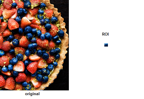
The first step for this process is to get a truecolor image and crop the ROI from the image. The following figure shows the image I have selected and the ROI.

Figure 3. All berries tart [3] and the ROI.

The RGB channels of the truecolor image sample is then transformed to normalized chromaticity coordinates (NCC). NCC are coordinates in a color space which can separate brightness and chromaticity. These are expressed as

Note that r+g+b = 1. We can then use only two coordinates and the remaining can be taken by the known values. For this case, r and g are used and b= 1-r-g. In the color space we will use, I tells the brightness and, r and g tells the chromaticity. We then call it r-g color space or NCC space. It is illustrated below

Figure 4. Normalized chromaticity chromaticity (NCC) space.

The said probability above involves the probability distribution function (PDF). It is actually the histogram normalized by the number of pixels of the ROI. For this case, the space has r and g. The joint PDF is therefore p(r)p(g) which tests the likelihood of a pixel to belong to the ROI. A Gaussian distribution can be used. Thus, the probability that a certain pixel with r chromaticity is a member of the ROI is expressed as

where μ_r and μ_g are the mean and σ_r and σ_g are the standard deviation from the R and G image channels. A similar way goes for the probability for a pixel with g chromaticity.  The joint PDF is the product of the two PDFs.

There are two ways to do color image segmentation: Parametric segmentation and Non-parametric segmentation.

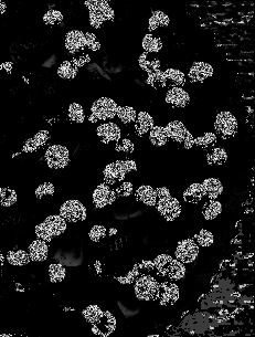
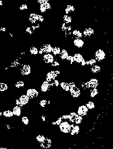
For parametric segmentation, the Gaussian PDF was used to segment the image. My segmented image is shown below.

Figure 5. Segmented Image using Parametric Segmentation.

Note: To clearly see the images, just click the image themselves.  😀

For the non-parametric segmentation, the 2D histogram of the ROI was used to determine whether the pixels belong to the ROI. It is shown below.

Figure 6. 2D histogram of the ROI from Figure 3.

To check whether my 2D histogram of the ROI is correct, I compared it with the NCC space from Figure 4. Since in images, the origin is in the upper right corner, the histogram should be rotated by 90 degrees. By doing so, we get the following figure.

 

 

And yes, comparing the above image with Figure 4, I think my histogram is correct. The colors are along the bluish, cyanish region since the ROI is a part of a blueberry.

To get the segmented image, backprojection is done. From the color histogram of Figure 6, the pixel location is assigned with a value equal to the histogram in NCC space. My generated segmented image is shown below.

Figure 7. Segmented Image using Parametric Segmentation.

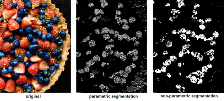
For better comparison, the original and segmented images are shown below.

Figure 8. Original and segmented images

From Figure 8, we can see that in general, non-parametric segmentation produced a more concrete segmented image. The segmented image using parametric segmentation actually uncovered more blueberries. It looks powdery but the shapes of the blueberries are more rendered. However, some of the black regions of the background were included in the segmentation. For non-parametric segmentation, some (very small areas) blueberries were hidden but the segmented image gave a higher similarity with the original images. The black background was not mistaken as part of the ROI (blueberry skin). The parametric segmentation gave clusters of points while the non-parametric segmentation gave shapes.

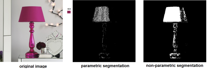
Here are some of image samples I used and processed. My observations were similar with those from Figure 8.

The original image above was obtained from reference [4]. Non-parametric segmentation won for this image type. 😉 I think it must be much better than parametric segmentation since histogram backprojection was used. Parametric segmentation assumed a Gaussian PDF which is not always the case so I think it won’t produce desirable results all the time.

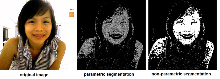
Ma’am Jing encouraged us to employ the newly taught image processing technique as face detector. The results are shown below. Non-parametric segmentation really gave a more detailed result.

I found segmentation techniques amazing because knowing that the ROI has dark pixels for the berries tart,  the generated segmented images were actually pleasing. The black background was not entirely tagged as part of the ROI.

For this activity, I give myself a grade of 10 for doing all of the steps on time (Yay!).

References:

1. Maricor Soriano, “A11  – Color Image Segmentation”, 2010.

2. “Image Segmentation”, retrieved from http://www.cs.cmu.edu/~jxiao/research.html.

3. “Berries & Tarts”, retrieved from http://4cakesinacup.com/page/4/.

4. “NtB Loves: Thinking Pink, Again”, retrieved from http://manolohome.com/2009/11/10/ntb-loves-thinking-pink-again/.

AP 186 Activity 10: Applications of Morphological Operations 3 of 3: Looping through Images

This activity involves determination of shape sizes in a binary image. This interesting activity can actually be extended to the detection of cancer cells in an image. Awesome right? *I so love AP 186!* Well, here’s how it was done.

The first step was to download the Circles002.jpg file which is an image containing scattered punched papers of the same size using a flatbed scanner. These cells were treated as cells imaged using a microscope. The goal of this step is to determine the best estimate of the cell size in pixel count given all the image processing techniques discussed in the previous activities.

It was also tasked that the determination of the cell size must be done by looping through subimages. Circles002.jpg was subdivided into 12 256×256 subimages using GIMP. Such subimages are shown below.

Note: In order to clearly see the images in this post, click on the image themselves.

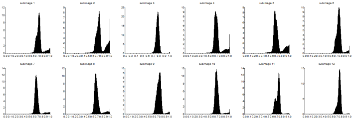
I made use of Scilab’s strcat function in order to loop though the images as I save them in one plot. This function has also enabled me to apply image processing techniques in the next sections in a faster way by means of indexing the filenames of the subimages and looping. Then I grayscaled each subimages and took their histograms. These are shown below.

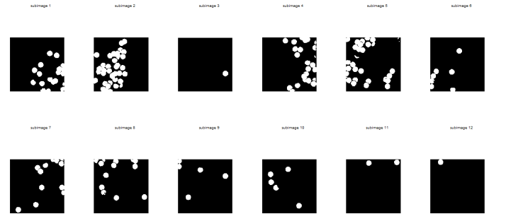
I took the threshold grayscale of each of the histograms that will make significant difference between the cells and the background. Using im2bw function of Scilab, I made use of the thresholds and converted the grayscale subimages to binary images. The binarized images are shown below. Notice that some of the images below contain white specks. I did not mind having these specks since I was aiming to establish a separation between the background and cells. The white specks will eventually be removed upon applying morphological operations.

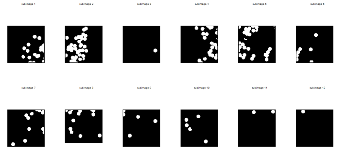
Most of the “cells” from the images above are actually overlapping. In order to distinguish one cell from another, the boundaries between them should be established. The concept of morphological operations can therefore be made use in this activity. The close and open operators can be used. Unfortunately, open is not available in SIP toolbox. But I have found out that its results can be produced upon applying dilate and then erode function of Scilab with a circular structuring element (SE). I chose to make use of such SE so that the circular shape of the cell can still be conserved.  Moreover, the close operator is equivalent to erode and then dilate functions.  The figure below shows the resulting images upon applying the equivalent operators for open operator. Notice that the subimages are cleaner now and the separations are more evident.

The next figure below shows the resulting images upon applying the equivalent operators for close operator. The boundaries between cells were not present in these subimages anymore so I chose the open operator for analyzing the blobs.

Note that edge detection can be used in distinguishing the shape of the cell. However, we are looking for the area of these cells in terms of pixel count. Edge detection is not applicable in this case.

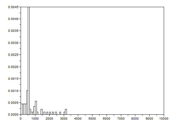
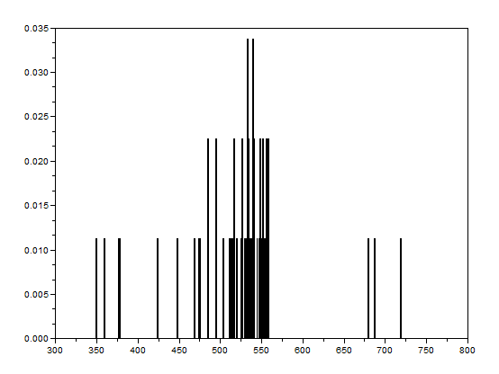
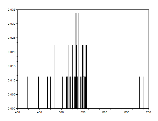
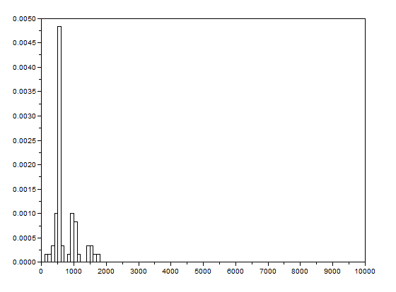
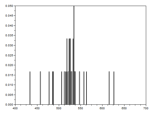
After that, the bwlabel function of Scilab was used to label the regions containing blobs. Blobs are the regions of interest (ROI) which are the isolated cells or those cells which are not overlapping. The area of a cell will be determined by counting the number of white pixels in that region containing such blobs. In other terms, the cell size is found out by means of counting the white pixels. It is applicable since the “cells” in the subimages have the same sizes. In order to know the number of white pixels, the histograms of these blobs were taken. The figure below shows the histograms of each of the blobs. The uppermost histogram has 10000 bins while the middle histogram shows the zoomed part with the x-axis ranging from 300 to 800. The lowermost histogram is also a zoomed portion with x values ranging from 400 to 700.

The best estimate of the area is 531 +- 42 pixels squared. This was calculated by summing the frequencies inside the interval [400,700] and using the mean and stdev functions of Scilab.

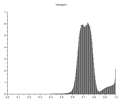
The second part of this activity involves the image entitled Circles with cancer.jpg. This is an image containing a set of punched papers of two sizes.  This part aims to let us design and implement a process that could isolate the larger cells (treated as cancer cells). I decide to redo the procedures (morphological operations) above but I ought not divide the image of interest into subimages. The following figure shows the grayscale image of Circles with cancer.jpg and its histogram.

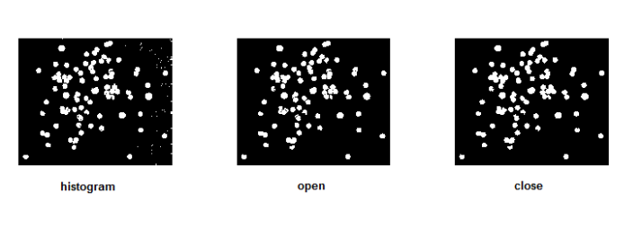
The SE in this case must be a circle again. However, this time it should be a little larger than the size of the “normal” cell, just a little bit so that it is smaller than a “cancer” cell. The figure below shows the binarized image with threshold value of 0.83 (leftmost), and the cleaned images using the equivalent SIP functions for open (middle) and close (rightmost) functions.

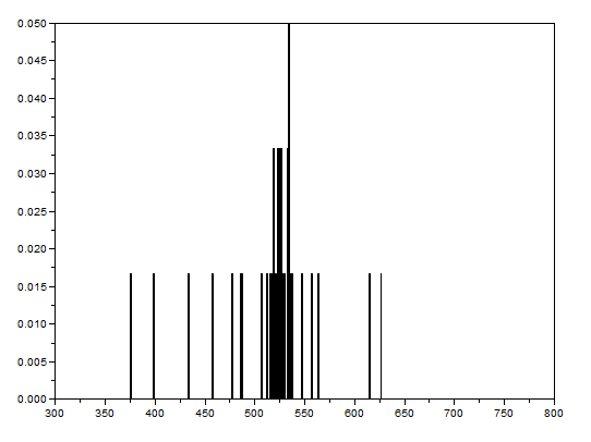
By histogram manipulation and bwlabel, the size and positions of the cancer cells were be determined. The histograms are shown below with different zoom levels similar in the previous histograms.

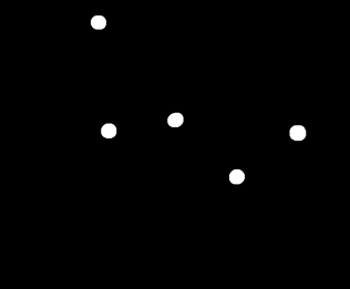
The best estimate of the cancer cell size by using the histogram is 884 +-56 pixels squared. The isolated cancers cells are shown below.

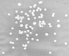
Hurrah! The best estimate for the cancer cell size is bigger than that of a normal cell. I think I got an acceptable answer. Morphological operations are really amazing! More importantly, the two raw images: Circles002.jpg (upper) and Circles with cancer.jpg (lower) are shown below.

Since the best estimate for the size of a normal cell was determined, we can tell whether a cell is abnormal or cancerous now. The purpose of using subimages in this case is to exercise us on how to process several samples.  I noticed that the processing for isolating the cancer cells took longer than the usual processing of images. But the result is worth waiting. In this activity, I will give myself a grade of 10 since I did every part with much enjoyment. :3

Reference:

1. Maricor Soriano, “A10-Applications of Morphological Operations 3 of 3: Looping through Images”, 2008.