Area estimation is quite common in land and such aspects can be calculated using GIS, remote sensing and other Geodetic instruments. It is utilized in so many ways, from land and bodies of water up to infinitesimal objects. We can estimate the area of everything we can see. The concern about the accuracy of calculation opens the door for mathematical and physical concepts. This activity involves area estimation by means of pixel counting via a binary image and Green’s theorem. Application of ratio and proportion is also required to transform pixel count to physical dimensions.
Primarily, I used Scilab 5.3.3 and SIVP toolbox for this activity. After a week of using them, an error showed up which tells that there is no Java update available and I can no longer open my Scilab 5.3.3. I uninstalled Scilab and installed it again. The same error occured so I decided to install an older version. I found Scilab 4.1.2 and it worked for me. I chose to install the SIP 0.4.0 toolbox because I cannot install the SIVP toolbox for this version and at the same time to save time.
I am really grateful that SIP 0.4.0 was an executable file so it was installed within Scilab in no time.
Since I started this activity using Scilab 5.3.3, the bitmap images of circle, square and triangles were already set. Unfortunately, Scilab 4.1.2 reads it as an indexed image containing only a single pixel value for all the pixels: 1. Everytime I execute imread, it displays the following results. This produces a plain white image instead of the image of a circle in a black background. *sob*

I was so frustrated because the basic function imread was not working 😦
It was instructed in the manual to save the image as BMP but my Scilab does not accept it. So I tried opening a truecolor image. It was successfully read and imshow-ed! Therefore, I tried drawing the circle, triangle and square in MS Paint and save them as PNG as an experiment. The function imread actually worked and imshow shows the correct image! Plus, the good thing is that Scilab 4.1.2 identified them as binary images! As for my case before, saving a black and white images as PNG is identified as truecolor image by Scilab 5.3.3. Scilab 4.1.2 is smarter this time and I think it will be fine to use PNG because the pixels are either 1 or 0 as i used imread. The result is shown below.

The same way went for my triangle and square images. The next step is to find the number of pixels in white. The following images shows the results for the circle, triangle and square samples.
![]()
This is the way to find the black pixels.
![]()
Hence, there are 203768 black pixels and 56328 white pixels for the circle, 185314 black pixels and 74782 white pixels for the square and 231575 black pixels and 28521 white pixels for the triangle. There are 512 x 508 pixels or 260096 pixels per image. By counting the number of white pixels, one can estimate the area of the white shapes by ratio and proportion just like what was done in Activity 1.
The next procedure is to get the coordinates of the pixels at the edge of the shapes in the images. Since I am using SIP toolbox, I used follow function to get the points. The coordinates are plotted and shown below

The purpose of getting the coordinates of edge pixels is to get the area of the shapes. The area can be calculated by implementing the discrete form of the Green’s Theorem. It is applicable since this activity deals with pixels of images. The discrete form of Green’s Theorem for the calculation of the area is:

where N_b is the total number of pixels at the edge of the shape or simply the boundary or contour of the shape, and x and y are the coordinates of these pixels. The corresponding Scilab code for this equation is shown below for the calculation of the area of the circle.

The resulting areas for each shape is shown below. The values are also compared with the analytical value.
Table 1. Calculate areas of the circle, square and triangle using the discrete form of the Green’s Theorem and analytic equations

From Table 1 it can be seen that the percent errors are small especially for the circle. If we focus on the analytic method, the percent error can still decrease by having a more precise value of pi in the computation of its area. The analytic solution for square should be of the rectangle form since the manner of drawing in MS Paint do not assure that the shape is square. Technically, and to be safe, it is considered as a rectangle. For the case of the triangle, it might be scalene so the analytical equation 0.5 x base x height would give an inexact area and made a bigger room for errors. More importantly, as the resolution of the images for the three shapes is increased, the distances of the vertices of the shapes will be closer and closer to the exact value so there will be minimal percent error.
The Scilab code used to compute for the analytical areas is shown below

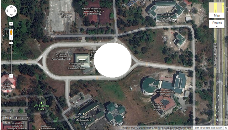
The last part of the activity is to look for a specific location in Google Maps and calculate for its area. I chose the UP College of Science Library and Administration Building (CSLAB). A satellite image of the building is shown below [1].

I then used MS Powerpoint to trace the CSLAB building. The I used MS Paint to check the pixel locations ratio of the pixels and the scale which can be seen at the lower left corner of the image above. The image below is the traced area of the CSLAB building which was calculated by following the discrete Green’s theorem discussed previously.

By Green’s theorem, the resulting area is 18394.5 pixels squared. The traced area of the image via the function follow and the Scilab code is shown below.

Using MS Paint, I have seen that for every 20 m in the map, there are 69 pixels. Thus, the ratio is 20 m: 69 pixels or 400 square meters: 4761 pixels squared. Therefore, the area of the CSLAB building in meters is 1545.43 square meters.
One cannot obtain the area if the given parameter is the pixel count from a binary image alone especially if the image is irregular in shape. Another way of estimating the area is by the geometry. Since the building is octagon, one can imagine a big square where its four corners are cut off (right triangles). Therefore, area of the octagon building is approximately equal to the area of a big square minus 4 right triangles.
The accuracy of the area calculated can be taken by looking at the literature value for the area of the CS building. However, it is not readily available in the web.
I give myself a grade of 10/10 for this activity since I have done the tasks required and as a credit to finish the activity after all the ‘sufferings’ I have encountered during installation.
References:
1. Google maps, retrieved from http://maps.google.com/.
2. Maricor Soriano, “A2 – Area Estimation for Images with Defined Edges”, Applied Physics 186 Laboratory Manual, 2012.
