We can still apply our Physics skills even when we are traveling, relaxing and even when we visit social sites and upload pictures. This is by enhancing the images that we take.
In this activity, the histogram P1(r) of a grayscale image is taken and manipulated and the resulting image is investigated. The cumulative distribution (CDF) is also discussed and utilized to perform such technique. It is defined as
where g is a dummy variable. A specific CDF is classified whether it can be an ideal standard for enhancing grayscale images. It is tested by using it as the desired CDF expressed as
where P2(z) is the probability distribution function (PDF) or the histogram of the grayscale image. In order to get the enhanced image, we let G(z) = T(r). Hence, we use the expression
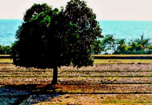
This technique is also known as the concept of backprojection of grayscale pixel values of the original PDF using a CDF of a desired PDF. The sample image I used was taken from San Fabian, Pangasinan when my family and I have gone to the beach. It is shown below.
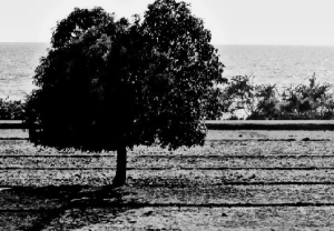
It is a 367 x 528-pixel truecolor image with a bit depth of 8 and these information were obtained using imfinfo of Scilab. Using gray_imread, the image above is converted to grayscale which is shown below.
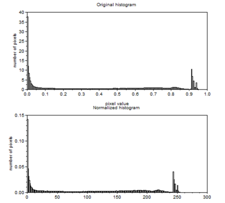
The main purpose of this activity is to enhance this image by means of changing the behavior of the histogram. The grayscale histogram of the image above is obtain using histplot. Upon using this function, the given pixel values were ranging from 0 to 1. I normalized the histogram so that the pixel values will range from 0 to 255. The two histograms are shown below.
From the histograms above, it can be observed that number of pixels in the middle of the histogram is almost flat and there are peaks for black and white pixels. This is acceptable since the image is grayscale and dark-colored. The maximum pixel value for the original histogram is 0.9611059 and 246.04311 for the normalized histogram. The minimum pixel value for both histograms is zero.
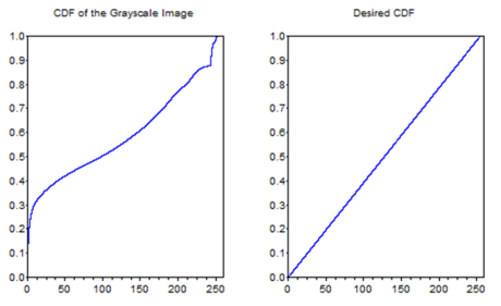
The Probability Distribution Function (PDF) here is the normalized histogram and the corresponding Cumulative Distribution Function (CDF) is shown below.
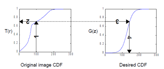
It can be seen from the image above that the CDF of the grayscale image is going up but does not follow the trend y = x. The desired CDF shown in the right of the image above is an example of a uniform distribution. This is the desired CDF which will be evaluated to check whether it can enhance the grayscale image. The enhanced image can be taken by backprojection or finding the corresponding y value of the image CDF in the desired CDF. The image below summarizes the said process.
The first step is to (1) find the CDF value of the grayscale image. The next step is to (2) trace and get the corresponding value in the desired CDF. (3) The position of the said pixel value is then taken and (4) the pixel in that position is replaced by the value of grayscale CDF [1].
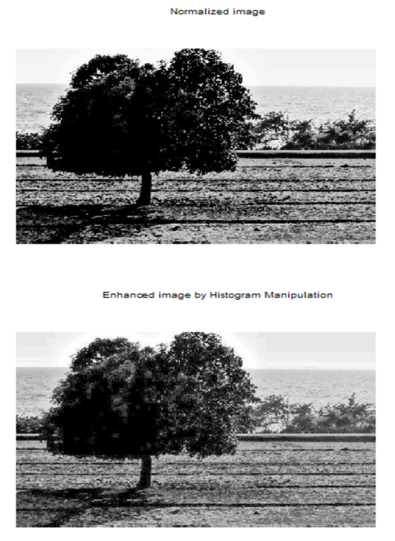
Using the straight increasing line as the desired CDF, the enhanced image of my grayscale image is shown below. The normalized grayscale image is also shown for comparison.
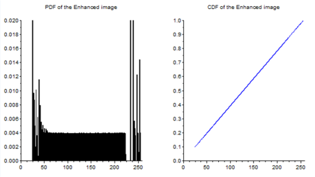
The enhanced image is really enhanced since the details of the dark regions of the original grayscale image were depicted upon modifying the histogram. Primarily, we thought of the dark region as shadow but actually there are important details that were uncovered upon doing histogram manipulation. This is one of the essence of using this kind of imaging technique. Moreover, there is also a bad effect of this image. If we look at the sky, the colors were sharpened and made it look pixelated. This is the consequence of unveiling or lightening the other parts of the image especially in the tree. The corresponding normalized histogram or the PDF and the CDF of the enhanced image above is also shown below in order to see the change in its distribution and its influence on the grayscale image. The enhanced image is called the histogram-equalized image.
The PDF above tell us that the values were quite near to each other this time compared to the histogram of the original grayscale image. This can be classified as a histogram-equalized image [1]. The difference between the black and white and middle-pixels were comparably smaller than before. The number of pixels with zero values in the original grayscale image was greater than 37. In the enhanced image, however, the number of zero-valued pixels was lower than 35. The number of white pixels also increased from zero up to ten upon executing backprojection. In this case, we can say that if the PDF has a flat distribution or the values are of nearly the same values or simply histogram-equalized, the image looks better than when the pixel values in the histogram have large differences.
Moreover, if we go back to the CDF of the normalized grayscale image, it can be seen that it is entirely different from the CDF of the enhanced image. The latter is perfectly linear and this is the result of a better-looking grayscale image. Hence, a straight increasing CDF is a good standard for producing an enhanced grayscale image.
It was noted stated that the human eye has a nonlinear response [1]. Hence, it was also tasked to make a nonlinear CDF which is considered to be the desired CDF and check whether the corresponding enhanced image is really enhanced when it is perceived by the human eye. The corresponding enhanced image is shown below.
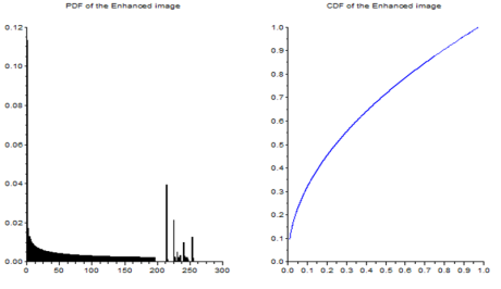
The processing of this image took about 20 mins or longer. The PDF and CDF of this enhanced image is shown below. It can be seen below that there are no pixel values with 0 values in the PDF and the CDF is nonlinear.
Comparing the two enhanced images, we can see that the backprojection using linear CDF has enhanced the original grayscale image more since it uncovered more hidden information. The image backprojected with a nonlinear CDF has uncovered lesser number of dark pixels. Thus, it has slightly enhanced the image. It is slightly darker than with the image with linear CDF but slightly lighter than the original grayscale image. Moreover, if we look at the background of the scene, the gradient of the colors are sharper especially the sky immediately around the tree. This makes the image look more pixelated than with the effect cause by the linear CDF.
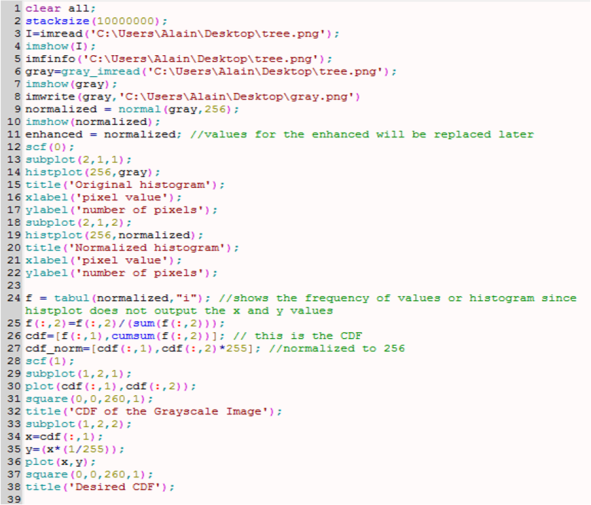
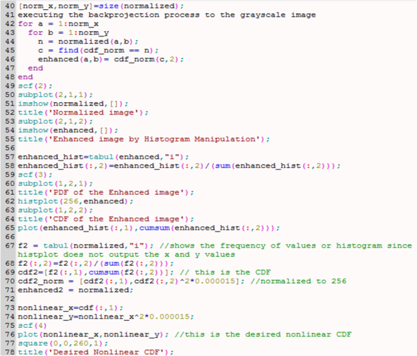
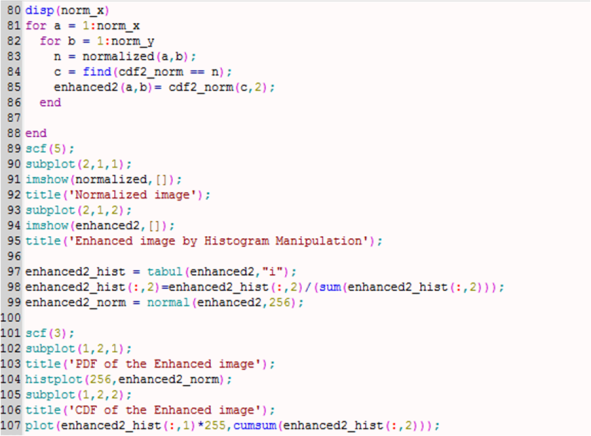
The Scilab code for processing the two enhanced images by linear and nonlinear CDF is shown below:
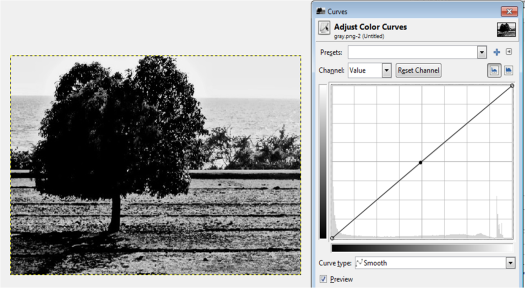
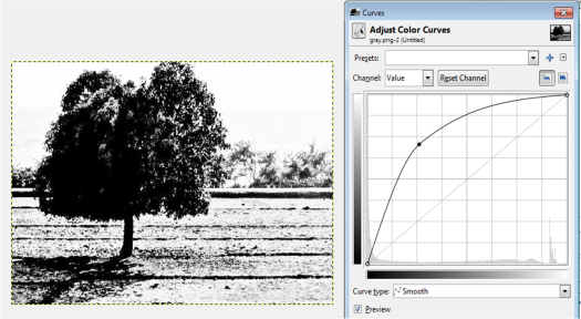
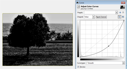
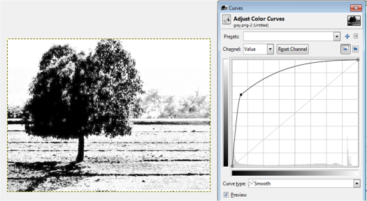
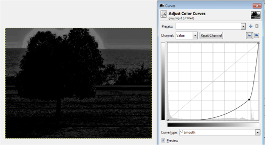
The histogram manipulation technique above can also be done in by image processing software like GIMP (GNU Image Manipulation Program). It is a freeware and can be downloaded from http://www.gimp.org. The CDF are manipulated by clicking the Colors menu and choosing Curves. The CDF manipulation and the “enhanced” images are shown below.
One thing I noticed about GIMP is that the initial CDF of the grayscale image was already an increasing line. Because of this, the enhanced images by this software are expected to be not exactly the same with the processed images by Scilab. By GIMP CDF manipulation, we can see that the region of the sky surrounding the tree has no gradient making the region look unrealistic. As the CDF is skewed to the right, the image becomes darker since the accumulated area slowly increases meaning there are more black pixels (PDF). On the other hand, if the CDF is skewed to the left, it implies a fast increase in the cumulative value and the values are in favor of white (255). The increasing line in this case is an acceptable image already. However, if we want to uncover more details about the tree and other plants around, the shadows should be eliminated. Hence, the CDF should be slightly moved to the left but not too much so that the image will not be saturated.
Another image processing software which can manipulate histogram and CDF is Histogram Manipulation Version 1.2.115.218 by Tomas Vondracek
from http://www.softsea.com/download/Histogram-Manipulation.html
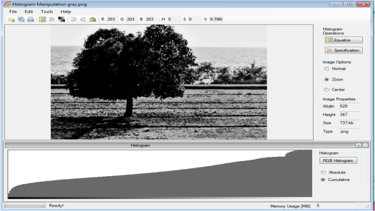
In this software, one can make the desired CDF by clicking the Specification button. Upon clicking, the histogram is manipulated using the mouse. The corresponding CDF is shown by choosing Cumulative. The original CDF of the grayscale image is shown below. It can be observed that this CDF is consistent with the CDF obtained using Scilab (I’m so happy!). ‘
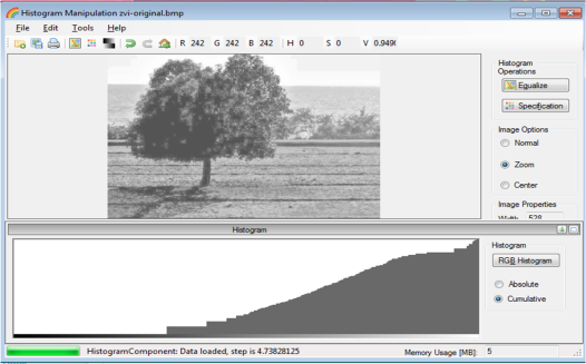
If the CDF is increasing and nonlinear like the one below, the grayscale image is more whitish but gives more details. This result is consistent with the results of GIMP.
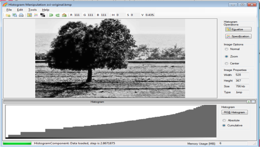
If the CDF is increasing more consistently, the image produced is more detailed without being too whitish and shadowy. The best image I could produce using this software is shown below. The CDF is increasing.
I give myself a grade of 10/10 for doing all the required steps.
References:
1. Maricor Soriano, “A5 – Enhancement by Histogram Manipulation 2010”, Applied Physics 186 Laboratory Manual, 2010.


